Schrödinger equation

2008/9 Schools Wikipedia Selection. Related subjects: Physics

Quantum mechanics

${\Delta x}\, {\Delta p} \ge \frac{\hbar}{2}$

Uncertainty principle

Mathematical formulation of...

Background
Classical mechanics Old quantum theory Interference · Bra-ket notation Hamiltonian

Fundamental concepts
Quantum state · Wave function Superposition · Entanglement Measurement · Uncertainty Exclusion · Duality Decoherence · Ehrenfest theorem · Tunneling

Experiments
Double-slit experiment Davisson–Germer experiment Stern–Gerlach experiment Bell's inequality experiment Popper's experiment Schrödinger's cat Elitzur-Vaidman bomb-tester Quantum eraser

Formulations
Schrödinger picture Heisenberg picture Interaction picture Matrix mechanics Sum over histories

Equations
Schrödinger equation Pauli equation Klein–Gordon equation Dirac equation

Interpretations
Copenhagen · Ensemble Hidden variable theory · Transactional Many-worlds · Consistent histories Quantum logic

Advanced topics
Quantum field theory Quantum gravity Theory of everything

Scientists
Planck · Einstein · Bohr · Sommerfeld · Kramers · Heisenberg· Born · Jordan · Pauli · Dirac · de Broglie · Schrödinger · von Neumann · Wigner · Feynman · Bohm · Everett · Bell

In physics, especially quantum mechanics, the Schrödinger equation is an equation that describes how the quantum state of a physical system changes in time. It is as central to quantum mechanics as Newton's laws are to classical mechanics.

In the standard interpretation of quantum mechanics, the quantum state, also called a wavefunction or state vector, is the most complete description that can be given to a physical system. Solutions to Schrödinger's equation describe atomic and subatomic systems, electrons and atoms, but also macroscopic systems, possibly even the whole universe. The equation is named after Erwin Schrödinger, who discovered it in 1926.

Schrödinger's equation can be mathematically transformed into Heisenberg's matrix mechanics, and into the Feynman's path integral formulation. The Schrödinger equation describes time in a way that is inconvenient for relativistic theories, a problem which is less severe in Heisenberg's formulation and completely absent in the path integral.

The Schrödinger equation

There are several different Schrödinger equations.

General quantum system

For a general quantum system:

$i\hbar {d\Psi \over dt} = \hat H \Psi$

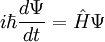
where

$ψ$ is the wavefunction, which is the probability amplitude for different configurations.
$\scriptstyle \hbar$ is Planck's constant over $2π$ , and it can be set to a value of 1 when using natural units.
$\scriptstyle \hat H$ is the Hamiltonian operator.

Single particle in three dimensions

For a single particle in three dimensions:

$i\hbar\frac{\partial}{\partial t} \psi = -\frac{\hbar^2}{2m}\nabla^2\psi + V(x,y,z)\psi$

where

$ψ$ is the wavefunction, which is the amplitude for the particle to have a given position at any given time.
$m$ is the mass of the particle.
$V (x, y, z)$ is the potential energy the particle has at each position.

Historical background and development

Einstein interpreted Planck's quanta as photons, particles of light, and proposed that the energy of a photon is proportional to its frequency, a mysterious wave-particle duality. Since energy and momentum are related in the same way as frequency and wavenumber in relativity, it followed that the momentum of a photon is proportional to its wavenumber.

DeBroglie hypothesized that this is true for all particles, for electrons as well as photons, that the energy and momentum of an electron are the frequency and wavenumber of a wave. Assuming that the waves travel roughly along classical paths, he showed that they form standing waves only for certain discrete frequencies, discrete energy levels which reproduced the old quantum condition.

Following up on these ideas, Schrödinger decided to find a proper wave equation for the electron. He was guided by Hamilton's analogy between mechanics and optics, encoded in the observation that the zero-wavelength limit of optics resembles a mechanical system--- the trajectories of light rays become sharp tracks which obey a principle of least action. Hamilton believed that mechanics was the zero-wavelength limit of wave propagation, but did not formulate an equation for those waves. This is what Schrödinger did, and a modern version of his reasoning is reproduced in the next section. The equation he found is (in natural units):

$i \frac{\partial}{\partial t}\psi=-\frac{1}{2m}\nabla^2\psi + V(x)\psi$

Using this equation, Schrödinger computed the spectral lines for hydrogen by treating a hydrogen atom's single negatively charged electron as a wave, $\psi\;$ , moving in a potential well, V, created by the positively charged proton. This computation reproduced the energy levels of the Bohr model.

But this was not enough, since Sommerfeld had already seemingly correctly reproduced relativistic corrections. Schrödinger used the relativistic energy momentum relation to find what is now known as the Klein-Gordon equation in a Coulomb potential:

$(E + {e^2\over r} )^2 \psi = - \nabla^2\psi + m^2 \psi$

He found the standing-waves of this relativistic equation, but the relativistic corrections disagreed with Sommerfeld's formula. Discouraged, he put away his calculations and secluded himself in an isolated mountain cabin with a lover.

While there, Schrödinger decided that the earlier nonrelativistic calculations were novel enough to publish, and decided to leave off the problem of relativistic corrections for the future. He put together his wave equation and the spectral analysis of hydrogen in a paper in 1926.. The paper was enthusiastically endorsed by Einstein, who saw the matter-waves as the visualizable antidote to what he considered to be the overly formal matrix mechanics.

The Schrödinger equation tells you the behaviour of $ψ$ , but does not say what $ψ$ is. Schrödinger tried unsuccessfully, in his fourth paper, to interpret it as a charge density. In 1926 Max Born, just a few days after Schrödinger's fourth and final paper was published, successfully interpreted $ψ$ as a probability amplitude. Schrödinger, though, always opposed a statistical or probabilistic approach, with its associated discontinuities; like Einstein, who believed that quantum mechanics was a statistical approximation to an underlying deterministic theory, Schrödinger was never reconciled to the Copenhagen interpretation.

Derivation

Short Heuristic Derivation

Assumptions

(1) The total energy E of a particle is

$E= T + V = \frac{p^2}{2m}+V$

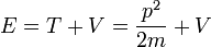
This is the classical expression for a particle with mass m where the total energy E is the sum of the kinetic energy, $\frac{p^2}{2m}$ , and the potential energy V. The momentum of the particle is p, or mass times velocity. The potential energy is assumed to vary with position, and possibly time as well.

Note that the energy E and momentum p appear in the following two relations:

(2) Einstein's light quanta hypothesis of 1905, which asserts that the energy E of a photon is proportional to the frequency f of the corresponding electromagnetic wave:

$E = h f = {h \over 2\pi} (2\pi f) = \hbar \omega \;$

where the frequency f of the quanta of radiation (photons) are related by Planck's constant h,

and $\omega = 2\pi f\;$ is the angular frequency of the wave.

(3) The de Broglie hypothesis of 1924, which states that any particle can be associated with a wave, represented mathematically by a wavefunction Ψ, and that the momentum p of the particle is related to the wavelength λ of the associated wave by:

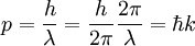
$p = { h \over \lambda } = { h \over 2\pi } {2\pi \over \lambda} = \hbar k\;$

where $\lambda\,$ is the wavelength and $k = 2\pi / \lambda\;$ is the wavenumber of the wave.

Expressing p and k as vectors, we have

$\mathbf{p} =\hbar \mathbf{k}\;$

Expressing the wave function as a complex plane wave

Schrödinger's great insight, late in 1925, was to express the phase of a plane wave as a complex phase factor:

$\Psi(\mathbf{x},t) = Ae^{i(\mathbf{k}\cdot\mathbf{x}- \omega t)} = Ae^{i \mathbf{k} \cdot \mathbf{x}}e^{-i\omega t} = \psi(\mathbf{x}) \phi(t)$

where

$\psi(\mathbf{x}) = Ae^{i \mathbf{k} \cdot \mathbf{x}}$

and

$\phi(t) = e^{-i\omega t} \,$

and to realize that since

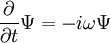
$\frac{\partial}{\partial t} \Psi = -i\omega \Psi$

then

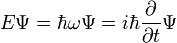
$E \Psi = \hbar \omega \Psi = i\hbar\frac{\partial}{\partial t} \Psi$

and similarly since:

$\frac{\partial}{\partial x} \Psi = i k_x \Psi$

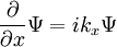
then

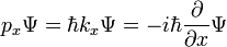
$p_x \Psi = \hbar k_x \Psi = -i\hbar\frac{\partial}{\partial x} \Psi$

and hence:

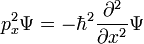
$p_x^2 \Psi = -\hbar^2\frac{\partial^2}{\partial x^2} \Psi$

so that, again for a plane wave, he obtained:

$p^2 \Psi = (p_x^2 + p_y^2 + p_z^2) \Psi = -\hbar^2\left(\frac{\partial^2}{\partial x^2} + \frac{\partial^2}{\partial y^2} + \frac{\partial^2}{\partial z^2}\right) \Psi = -\hbar^2\nabla^2 \Psi$

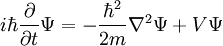
And by inserting these expressions for the energy and momentum into the classical formula we started with we get Schrödinger's famed equation for a single particle in the 3-dimensional case in the presence of a potential V:

$i\hbar\frac{\partial}{\partial t}\Psi=-\frac{\hbar^2}{2m}\nabla^2\Psi + V\Psi$

Longer Discussion

The particle is described by a wave, and in natural units, the frequency is the energy E of the particle, while the momentum p is the wavenumber k. These are not two separate assumptions, because of special relativity.

$E= \omega \;\;\;\;P=k \,$

The total energy is the same function of momentum and position as in classical mechanics:

$E = T(p) + V(x) = {p^2\over 2m} + V(x)$

where the first term T(p) is the kinetic energy and the second term V(x) is the potential energy.

Schrödinger required that a Wave packet at position x with wavenumber k will move along the trajectory determined by Newton's laws in the limit that the wavelength is small.

Consider first the case without a potential, V=0.

$E = {1\over 2m} (p_x^2+p_y^2 + p_z^2)$

$\omega = {1\over 2m} (k_x^2 + k_y^2 + k_z^2)$

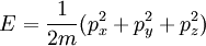
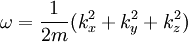
So that a plane wave with the right energy/frequency relationship obeys the free Schrodinger equation:

$i {\partial \over \partial t} \psi = -{1 \over 2m} ( {\partial^2 \psi \over \partial x^2} + {\partial^2 \psi \over \partial y^2} + {\partial^2 \psi \over \partial z^2} )$

and by adding together plane waves, you can make an arbitrary wave.

When there is no potential, a wavepacket should travel in a straight line at the classical velocity. The velocity v of a wavepacket is:

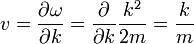
$v = {\partial \omega \over \partial k } = {\partial \over \partial k} { k^2\over 2m} = { k\over m}$

which is the momentum over the mass as it should be. This is one of Hamilton's equations from mechanics:

${dx \over dt} = {\partial H \over \partial p}$

after identifying the energy and momentum of a wavepacket as the frequency and wavenumber.

To include a potential energy, consider that as a particle moves the energy is conserved, so that for a wavepacket with approximate wavenumber k at approximate position x the quantity

${ k^2\over 2m } + V(x)$

must be constant. The frequency doesn't change as a wave moves, but the wavenumber does. So where there is a potential energy, it must add in the same way:

$i{\partial \over \partial t}\psi=-{1\over 2m}\nabla^2\psi + V(x)\psi$

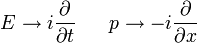
This is the time dependent schrodinger equation. It is the equation for the energy in classical mechanics, turned into a differential equation by substituting:

$E\rightarrow i{\partial\over \partial t} \;\;\;\;\;\; p\rightarrow -i{\partial\over \partial x}$

Schrödinger studied the standing wave solutions, since these were the energy levels. Standing waves have a complicated dependence on space, but vary in time in a simple way:

$\psi(x,t) = \psi(x) e^{- iEt } \,$

substituting, the time-dependent equation becomes the standing wave equation:

${E}\psi(x) = - {1\over 2m} \nabla^2 \psi(x) + V(x) \psi(x)$

Which is the original time-independent Schrodinger equation.

In a potential gradient, the k-vector of a short-wavelength wave must vary from point to point, to keep the total energy constant. Sheets perpendicular to the k-vector are the wavefronts, and they gradually change direction, because the wavelength is not everywhere the same. A wavepacket follows the shifting wavefronts with the classical velocity, with the acceleration equal to the force divided by the mass.

an easy modern way to verify that Newton's second law holds for wavepackets is to take the Fourier transform of the time dependent Schrodinger equation. For an arbitrary polynomial potential this is called the Schrodinger equation in the momentum representation:

$i{\partial \psi(p) \over \partial t} = {p^2\over 2m} \psi(p) + V(i{\partial\over \partial x}) \psi(p)$

The group-velocity relation for the fourier trasformed wave-packet gives the second of Hamilton's equations.

${dp \over dt} = -{\partial H \over \partial x}$

Versions

There are several equations which go by Schrodinger's name:

Time Dependent Equation

This is the equation of motion for the quantum state. In the most general form, it is written:

$i{d\over dt} \psi = \hat H \psi$

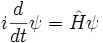
Where $\hat H$ is a linear operator acting on the wavefunction $ψ$ . $\hat H$ takes as input one $ψ$ and produces another in a linear way, a function-space version of a matrix multiplying a vector. For the specific case of a single particle in one dimension moving under the influence of a potential V:

$i{d\over dt} \psi = -{1\over 2m} {\partial^2 \over \partial x^2} \psi(x) + V(x) \psi(x) \,$

and the operator H can be read off:

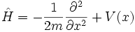
$\hat H = -{1\over 2m} {\partial^2 \over \partial x^2} + V(x) \,$

it is a combination of the operator which takes the second derivative, and the operator which pointwise multiplies $ψ$ by V(x). When acting on $ψ$ it reproduces the right hand side.

For a particle in three dimensions, the only difference is more derivatives:

$i{d\over dt} \psi = -{1\over 2m} \nabla^2 \psi + V(x) \psi \,$

and for N particles, the difference is that the wavefunction is in 3N-dimensional configuration space, the space of all possible particle positions.

$i{d\over dt} \psi(x_1,...,x_n) = (-{\nabla_1^2\over 2m_1} - {\nabla_2^2 \over 2m_2} ... - {\nabla_N^2\over 2m_N} ) \psi + V(x_1,..,x_N)\psi \,$

This last equation is in a very high dimension, so that the solutions are not easy to visualize.

Time Independent Equation

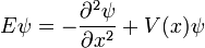
This is the equation for the standing waves, the eigenvalue equation for H. In abstract form, for a general quantum system, it is written:

$E \psi = \hat H \psi \,$

For a particle in one dimension, with the mass absorbed into rescaling either time or space:

$E \psi = -{\partial^2 \psi \over \partial x^2} + V(x)\psi \,$

But there is a further restriction--- the solution must not grow at infinity, so that it has a finite norm:

$|| \psi ||^2 = \int_x \psi^*(x) \psi(x) \,$

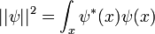
For example, when there is no potential, the equation reads:

$- E \psi = {\partial^2 \psi \over \partial x^2} \,$

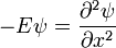
which has oscillatory solutions for E>0 (the C's are arbitrary constants):

$\psi_E(x) = C_1 e^{i\sqrt{E} x} + C_2 e^{-i\sqrt{E}x} \,$

and exponential solutions for E<0

$\psi_{-|E|}(x) = C_1 e^{\sqrt{|E|} x} + C_2 e^{-\sqrt{|E|} x} \,$

The exponentially growing solutions have an infinite norm, and are not physical. They are not allowed in a finite volume with periodic or fixed boundary conditions.

For a constant potential V the solution is oscillatory for E>V and exponential for E<V, corresponding to energies which are allowed or disallowed in classical mechnics. Oscillatory solutions have a classically allowed energy and correspond to actual classical motions, while the exponential solutions have a disallowed energy and describe a small amount of quantum bleeding into the classically disallowed region, to quantum tunneling. If the potential V grows at infinity, the motion is classically confined to a finite region, which means that in quantum mechanics every solution becomes an exponential far enough away. The condition that the exponential is decreasing restricts the energy levels to a discrete set, called the allowed energies.

Energy Eigenstates

A solution $\scriptstyle \psi_E(x)$ of the time independent equation is called an energy eigenstate with energy E:

$H\psi_E = E \psi_E \,$

To find the time dependence of the state, consider starting the time-dependent equation with an initial condition $ψ E (x)$ . The time derivative at t=0 is everywhere proportional to the value:

$i {d\over dt} \psi(x) = H \psi(x) = E \psi(x) \,$

So that at first the whole function just gets rescaled, and it maintains the property that its time derivative is proportional to itself. So for all times,

$\psi(x,t) = A(t) \psi_E(x) \,$

substituting,

$i {dA \over dt } = - E A \,$

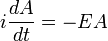
So that the solution of the time-dependent equation with this initial condition is:

$\psi(x,t) = \psi_E(x) e^{-iEt} \,$

or, with explicit $\scriptstyle\hbar$ s.

$\psi(x,t) = \psi_E(x) e^{-i{E t\over\hbar}} \,$

This is a restatement of the fact that solutions of the time-independent equation are the standing wave solutions of the time dependent equation. They only get multiplied by a phase as time goes by, and otherwise are unchanged.

Superpositions of energy eigenstates change their properties according to the relative phases between the energy levels.

Properties

First Order in Time

The Schrodinger equation describes the time evolution of a quantum state, and must determine the future value from the present value. A classical field equation can be second order in time derivatives, the classical state can include the time derivative of the field. But a quantum state is a full description of a system, so that the Schrodinger equation is always first order in time.

Linear

The Schrödinger equation is linear in the wavefunction: if $ψ(x, t)$ and $φ(x, t)$ are solutions to the time dependent equation, then so is $a ψ + b φ$ , where a and b are any complex numbers.

In quantum mechanics, the time evolution of a quantum state is always linear, for fundamental reasons. Although there are nonlinear versions of the Schrodinger equation, these are not equations which describe the evolution of a quantum state, but classical field equations like Maxwell's equations or the Klein-Gordon equation.

The Schrodinger equation itself can be thought of as the equation of motion for a classical field not for a wavefunction, and taking this point of view, it describes a coherent wave of nonrelativistic matter, a wave of a Bose condensate or a superfluid with a large indefinite number of particles and a definite phase and amplitude.

Real Eigenstates

The time-independent equation is also linear, but in this case linearity has a slightly different meaning. If two wavefunctions $ψ 1$ and $ψ 2$ are solutions to the time-independent equation with the same energy E, then any linear combination of the two is a solution with energy E. Two different solutions with the same energy are called degenerate.

$\hat H (a\psi_1 + b \psi_2 ) = ( a \hat H \psi_1 + b \hat H \psi_2) = E (a \psi_1 + b\psi_2) \,$

In an arbitrary potential, there is one obvious degeneracy: if a wavefunction $ψ$ solves the time-independent equation, so does $ψ *$ . By taking linear combinations, the real and imaginary part of $ψ$ are each solutions. So that restricting attention to real valued wavefunctions does not affect the time-independent eigenvalue problem.

In the time-dependent equation, complex conjugate waves move in opposite directions. Given a solution to the time dependent equation $ψ(x, t)$ , the replacement:

$\psi(x,t) \rightarrow \psi^*(x,-t) \,$

produces another solution, and is the extension of the complex conjugation symmetry to the time-dependent case. The symmetry of complex conjugation is called time-reversal.

Unitary Time Evolution

The Schrodinger equation is Unitary, which means that the total norm of the wavefunction, the sum of the squares of the value at all points:

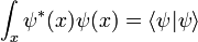
$\int_x \psi^*(x) \psi(x) = \langle \psi | \psi \rangle \,$

has zero time derivative.

The derivative of $ψ *$ is according to the complex conjugate equations

$-i \hbar {d\over dt} \psi^* = \hat H^\dagger \psi^* \,$

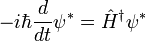
where the operator $H^\dagger$ is defined as the continuous analog of the Hermitian conjugate,

$\langle \eta H^{\dagger} | \psi \rangle = \langle \eta | H \psi \rangle \,$

For a discrete basis, this just means that the matrix elements of the linear operator H obey:

$\hat H_{ij} = \hat H^*_{ji} \,$

The derivative of the inner product is:

${d\over dt} \langle \psi | \psi \rangle = i \langle \psi \hat H^\dagger | \psi \rangle - i \langle \psi| H \psi \rangle \,$

and is proportional to the imaginary part of H. If H has no imaginary part, if it is self-adjoint, then the probability is conserved. This is true not just for the Schrodinger equation as written, but for the Schrodinger equation with nonlocal hopping:

$i{d \over dt} \psi(x) = \int_y H(x,y) \psi(y) \,$

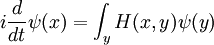
so long as:

$H(x,y) = H(y,x)^* \,$

the particular choice:

$H(x,y) = - {1\over 2m} \nabla_x^2 \delta(x-y) + V(x) \delta(x-y) \,$

reproduces the local hopping in the ordinary Schrodinger equation. On a discrete lattice approximation to a continuous space, H(x,y) has a simple form:

$H(x,y) = -{1\over 2m} \,$

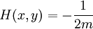
whenever x and y are nearest neighbors. On the diagonal

$H(x,x) = +{n\over 2m} + V(x) \,$

where n is the number of nearest neighbors.

Positive Energies

The solutions of the Schrodinger equation in a potential which is bounded below have a frequency which is bounded below. For any linear operator $\scriptstyle \hat A$ , the smallest eigenvector minimizes the quantity:

$\langle \psi |A|\psi \rangle$

over all $ψ$ which are normalized:

by the variational principle.

The value of the energy for the Schrodinger Hamiltonian is then the minimum value of:

$\langle \psi|H|\psi\rangle = \int_x \psi^*(x) (- \nabla^2 \psi + V(x)\psi) = \int_x |\nabla \psi|^2 + V(x) |\psi|^2 dx$

after an integration by parts, and the right hand side is positive definite when V is positive.

Positive Definite Nondegenerate Ground State

For potentials which are bounded below and are not infinite over a region, there is a ground state which minimizes the integral above. This lowest energy wavefunction is real and positive definite.

Suppose for contradiction that $ψ$ is a lowest energy state and has a sign change, then $η(x) = | ψ(x) |$ , the absolute value of $ψ$ obeys

$V(x)|\eta|^2 = V(x)|\psi|^2\,$

everywhere, and

$|\nabla \eta|^2 = |\nabla \psi|^2$

except for a set of measure zero. So $η$ is also a minimimum of the integral, and it has the same value as $ψ$ . But by smoothing out the bends at the sign change, the gradient contribution to the integral is reduced while the potential energy is hardly altered, so the energy of $η$ can be reduced, which is a contradiction.

The lack of sign changes also proves that the ground state is nondegenerate, since if there were two ground states with energy E which were not proportional to each other, a linear combination of the two would also be a ground state with a zero.

These properties allow the analytic continuation of the Schrodinger equation to be identified as a stochastic process, which can be represented by a path integral.

Completeness

The energy eigenstates form a basis--- any wavefunction may be written as a sum over the discrete energy states or an integral over continuous energy states, or more generally as an integral over a measure. This is the spectral theorem in mathematics, and in a finite state space it is just a statement of the completeness of the eigenvectors of a Hermitian matrix.

Local Conservation of Probability

The probability density of a particle is $ψ * (x)ψ(x)$ . The probability flux is defined as:

$\mathbf{j} = {\hbar \over m} \cdot {1 \over {2 \mathrm{i}}} \left( \psi ^{*} \nabla \psi - \psi \nabla \psi^{*} \right) = {\hbar \over m} \operatorname{Im} \left( \psi ^{*} \nabla \psi \right)$

in units of (probability)/(area × time).

The probability flux satisfies the continuity equation:

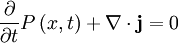
${ \partial \over \partial t} P\left(x,t\right) + \nabla \cdot \mathbf{j} = 0$

where $P\left(x, t\right)$ is the probability density and measured in units of (probability)/(volume) = r⁻³. This equation is the mathematical equivalent of the probability conservation law.

For a plane wave:

$\psi (x,t) = \, A e^{ \mathrm{i} (k x - \omega t)}$

$j\left(x,t\right) = \left|A\right|^2 {\hbar k \over m}$

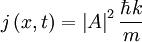
So that not only is the probability of finding the particle the same everywhere, but the probability flux is as expected from an object moving at the classical velocity $p / m$ .

The reason that the Schrodinger equation admits a probability flux is because all the hopping is local and forward in time.

Heisenberg Observables

There are many linear operators which act on the wavefunction, each one defines a Heisenberg matrix when the energy eigenstates are discrete. For a single particle, the operator which takes the derivative of the wavefunction in a certain direction:

$\hat p = {i\hbar {\partial \over \partial x}}$

Is called the momentum operator. Multiplying operators is just like multiplying matrices, the product of A and B acting on $ψ$ is A acting on the output of B acting on $ψ$ .

An eigenstate of p obeys the equation:

$\hat p \psi = k \psi \,$

for a number k, and for a normalizable wavefunction this restricts k to be real, and the momentum eigenstate is a wave with frequency k.

$\psi(x) = e^{i kx} \,$

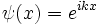
The position operator x multiplies each value of the wavefunction at the position x by x:

$\hat x(\psi) = x\psi$

So that in order to be an eigenstate of x, a wavefunction must be entirely concentrated at one point:

$\hat x \delta(x-x_0) = x_0 \delta(x-x_0)$

In terms of p, the Hamiltonian is:

$\hat H = {\hat p^2\over 2m} + V(x)$

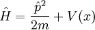
It is easy to verify that p acting on x acting on psi:

$\hat p (\hat x( \psi)) = -i \hbar {\partial \over \partial x}( x \psi) = -i x {\partial \over \partial x}\psi -i\hbar \psi$

while x acting on p acting on psi reproduces only the first term:

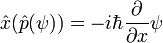
$\hat x(\hat p (\psi)) = -i \hbar {\partial \over \partial x} \psi$

so that the difference of the two is not zero:

$( x p - p x ) \psi = i \hbar \psi \,$

or in terms of operators:

$[x,p] = xp - px = i \hbar \,$

since the time derivative of a state is:

$i{d \over dt} \psi = \hat H \psi \,$

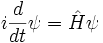
while the complex conjugate is

$- i{d\over dt} \psi^* = \hat H \psi^* \,$

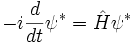
The time derivative of a matrix element

${d\over dt} \langle \eta | A |\psi \rangle = - \eta \hat H A \psi + \eta AH \psi = [H,A] \,$

obeys the Heisenberg equation of motion. This establishes the equivalence of the Schrodinger and Heisenberg formalisms, ignoring the mathematical fine points of the limiting procedure for continuous space.

Correspondence principle

The Schrödinger equation satisfies the correspondence principle. In the limit of small wavelength wavepackets, it reproduces Newton's laws. This is easy to see from the equivalence to matrix mechanics.

All operators in Heisenberg's formalism obey the quantum analog of Hamilton's equations:

${dA \over dt} = -i\hbar (AH - HA)$

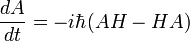
So that in particular, the equations of motion for the X and P operators are:

${dX \over dt} = {P\over m}$

${dP \over dt} = - {\partial V \over \partial x}$

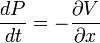
in the Schrodinger picture, the interpretation of this equation is that it gives the time rate of change of the matrix element between two states when the states change with time. Taking the expectation value in any state shows that Newton's laws hold not only on average, but exactly, for the quantities:

$\langle X\rangle = \int_x \psi^*(x)\psi(x) X = \langle \psi|X|\psi \rangle \,$

$\langle P\rangle = \int_x \psi^*(x) i\hbar {\partial \psi \over \partial x}(x) = \langle \psi |P|\psi\rangle \,$

Relativity

The Schrödinger equation does not take into account relativistic effects, as a wave equation, it is invariant under a Galilean transformation, but not under a Lorentz transformation. But in order to include relativity, the physical picture must be altered in a radical way.

A naive generalization of the Schrodinger equation uses the relativistic mass-energy relation (in natural units):

$E^2 = P^2 + m^2 \,$

to produce the differential equation:

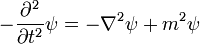
$- {\partial^2 \over \partial t^2}\psi = - \nabla^2 \psi + m^2 \psi \,$

which is relativistically invariant, but second order in $ψ$ , and so cannot be an equation for the quantum state. This equation also has the property that there are solutions with both positive and negative frequency, a plane wave solution obeys:

$\omega^2 - k^2 = m^2 \,$

which has two solutions, one with positive frequency the other with negative frequency. This is a disaster for quantum mechanics, because it means that the energy is unbounded below.

A more sophisticated attempt to solve this problem uses a first order wave equation, the Dirac equation, but again there are negative energy solutions. In order to solve this problem, it is essential to go to a multiparticle picture, and to consider the wave equations as equations of motion for a quantum field, not for a wavefunction.

The reason is that relativity is incompatible with a single particle picture. A relativistic particle cannot be localized to a small region without the particle number becoming indefinite. When a particle is localized in a box of length L, the momentum is uncertain by an amount roughly proportional to h/L by the uncertainty principle. This leads to an energy uncertainty of hc/L, when |p| is large enough so that the mass of the particle can be neglected. This uncertainty in energy is equal to the mass-energy of the particle when

$L = {\hbar \over mc} \,$

and this is called the Compton wavelength. Below this length, it is impossible to localize a particle and be sure that it stays a single particle, since the energy uncertainty is large enough to produce more particles from the vacuum by the same mechanism that localizes the original particle.

But there is another approach to relativistic quantum mechanics which does allow you to follow single particle paths, and it was discovered within the path-integral formulation. If the integration paths in the path integral include paths which move both backwards and forwards in time as a function of their own proper time, it is possible to construct a purely positive frequency wavefunction for a relativistic particle. This construction is appealing, because the equation of motion for the wavefunction is exactly the relativistic wave equation, but with a nonlocal constraint that separates the positive and negative frequency solutions. The positive frequency solutions travel forward in time, the negative frequency solutions travel backwards in time. In this way, they both analytically continue to a statistical field correlation function, which is also represented by a sum over paths. But in real space, they are the probability amplitudes for a particle to travel between two points, and can be used to generate the interaction of particles in a point-splitting and joining framework. The relativistic particle point of view is due to Richard Feynman.

Feynman's method also constructs the theory of quantized fields, but from a particle point of view. In this theory, the equations of motion for the field can be interpreted as the equations of motion for a wavefunction only with caution--- the wavefunction is only defined globally, and in some way related to the particle's proper time. The notion of a localized particle is also delicate--- a localized particle in the relativistic particle path integral corresponds to the state produced when a local field operator acts on the vacuum, and exacly which state is produced depends on the choice of field variables.

Solutions

Some general techniques are:

Perturbation theory
The variational principle
Quantum Monte Carlo methods
Density functional theory
The WKB approximation and semi-classical expansion

In some special cases, special methods can be used:

List of quantum mechanical systems with analytical solutions
Hartree-Fock method and post Hartree-Fock methods
Discrete delta-potential method

Free Schrödinger equation

When the potential is zero, the Schrödinger equation is linear with constant coefficients:

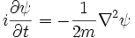
$i \frac{\partial \psi}{\partial t}=-{1\over 2m}\nabla^2\psi$

where $\scriptstyle \hbar$ has been set to 1. The solution $ψ t (x)$ for any initial condition $ψ 0 (x)$ can be found by Fourier transforms. Because the coefficients are constant, an initial plane wave:

$\psi_0(x) = A e^{i k x} \,$

stays a plane wave. Only the coefficient changes. Substituting:

${dA \over dt} = -{i k^2 \over 2m} A \,$

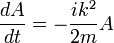
So that A is also oscillating in time:

$A(t) = A e^{- i {k^2 \over 2m} t} \,$

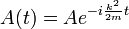
and the solution is:

$\psi_t(x) = A e^{i k x - i \omega t} \,$

Where $ω = k 2 / 2 m$ , a restatement of DeBroglie's relations.

To find the general solution, write the initial condition as a sum of plane waves by taking its Fourier transform:

$\psi_0(x) = \int_k \psi(k) e^{ikx} \,$

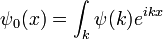
The equation is linear, so each plane waves evolves independently:

$\psi_t(x) = \int_k \psi(k)e^{-i\omega t} e^{ikx} \,$

Which is the general solution. When complemented by an effective method for taking Fourier transforms, it becomes an efficient algorithm for finding the wavefunction at any future time--- Fourier transform the initial conditions, multiply by a phase, and transform back.

Gaussian Wavepacket

An easy and instructive example is the Gaussian wavepacket:

$\psi_0(x) = e^{-x^2 / 2a} \,$

where a is a positive real number, the square of the width of the wavepacket. The total normalization of this wavefunction is:

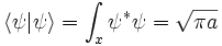
$\langle \psi|\psi\rangle = \int_x \psi^* \psi = \sqrt{\pi a}$

The Fourier transform is a Gaussian again in terms of the wavenumber k:

$\psi_0(k) = (2\pi a)^{d/2} e^{- a k^2/2} \,$

With the physics convention which puts the factors of $2π$ in Fourier transforms in the k-measure.

$\psi_0(x) = \int_k \psi_0(k) e^{-ikx} = \int {d^dk \over (2\pi)^d} \psi_0(k) e^{-ikx}$

Each separate wave only phase-rotates in time, so that the time dependent Fourier-transformed solution is:

$\psi_t(k) = (2\pi a)^{d/2} e^{- a { k^2\over 2} - it {k^2\over 2m}} = (2\pi a)^{d/2} e^{-(a+it/m){k^2\over 2}} \,$

The inverse Fourier transform is still a Gaussian, but the parameter a has become complex, and there is an overall normalization factor.

$\psi_t(x) = \left({a \over a + i t/m}\right)^{d/2} e^{- {x^2\over 2(a + i t/m)} } \,$

The branch of the square root is determined by continuity in time--- it is the value which is nearest to the positive square root of a. It is convenient to rescale time to absorb m, replacing t/m by t.

The integral of $ψ$ over all space is invariant, because it is the inner product of $ψ$ with the state of zero energy, which is a wave with infinite wavelength, a constant function of space. For any energy state, with wavefunction $η(x)$ , the inner product: