Global climate model
2008/9 Schools Wikipedia Selection. Related subjects: Climate and the Weather
General Circulation Models (GCMs) are a class of computer-driven models for weather forecasting, understanding climate and projecting climate change, where they are commonly called Global Climate Models. Versions designed for decade to century time scale climate applications were originally created by Syukuro Manabe and Kirk Bryan at the Geophysical Fluid Dynamics Laboratory in Princeton, New Jersey. These computationally intensive numerical models are based on the integration of a variety of fluid dynamical, chemical, and sometimes biological equations.
Atmospheric vs Ocean models
There are both atmospheric GCMs (AGCMs) and oceanic GCMs (OGCMs). An AGCM and an OGCM can be coupled together to form an atmosphere-ocean coupled general circulation model (AOGCM). With the addition of other components (such as a sea ice model or a model for evapotranspiration over land), the AOGCM becomes the basis for a full climate model. Within this structure, different variations can exist, and their varying response to climate change may be studied (e.g., Sun and Hansen, 2003).
Modeling trends: Carbon and Sulphur Cycle
A recent trend in GCMs is to extend them to become Earth system models, that include such things as submodels for atmospheric chemistry or a carbon cycle model to better predict changes in carbon dioxide concentrations resulting from changes in emissions. In addition this approach allows feedback between these systems to be taken into account. For example, Chemistry-Climate models allow the possible effects of climate change on the recovery of the ozone hole to be studied.
Climate prediction uncertainties depend on uncertainties in both models and the future course of industrial growth and technology (which is currently the largest unknown) (see IPCC scenarios below). Progress has been made in incorporating more realistic physics in the models, but significant uncertainties and unknowns remain.
Note that many simpler levels of climate model exist; some are of only heuristic interest; others continue to be scientifically relevant.
Model structure
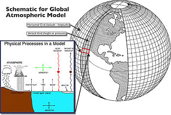
Three-dimensional (more properly four-dimensional) GCMs discretise the equations for fluid motion and integrate these forward in time. They also contain parametrisations for processes - such as convection - that occur on scales too small to be resolved directly. More sophisticated models may include representations of the carbon and other cycles.
A simple general circulation model (SGCM), a minimal GCM, consists of a dynamical core that relates material properties such as temperature to dynamical properties such as pressure and velocity. Examples are codes that solve the primitive equations, given energy input into the model, and energy dissipation in the form of scale-dependent friction, so that atmospheric waves with the highest wavenumbers are the ones most strongly attenuated. Such models may be used to study atmospheric processes within a simplified framework but are not suitable for future climate projections.
Atmospheric GCMs (AGCMs) model the atmosphere (and typically contain a land-surface model as well) and impose sea surface temperatures (SSTs). A large amount of information including model documentation is available from AMIP . They may include atmospheric chemistry.
- AGCMs consist of a dynamical core which integrates the equations of fluid motion, typically for:
- surface pressure
- horizontal components of velocity in layers
- temperature and water vapor in layers
- There is generally a radiation code, split into solar/short wave and terrestrial/infra-red/long wave
- Parametrizations are used to include the effects of various processes. All modern AGCMs include parameterizations for:
A GCM contains a number of prognostic equations that are stepped forward in time (typically winds, temperature, moisture, and surface pressure) together with a number of diagnostic equations that are evaluated from the simultaneous values of the variables. As an example, pressure at any height can be diagnosed by applying the hydrostatic equation to the predicted surface pressure and the predicted values of temperature between the surface and the height of interest. The pressure diagnosed in this way then is used to compute the pressure gradient force in the time-dependent equation for the winds.
Oceanic GCMs (OGCMs) model the ocean (with fluxes from the atmosphere imposed) and may or may not contain a sea ice model. For example, the standard resolution of HadOM3 is 1.25 degrees in latitude and longitude, with 20 vertical levels, leading to approximately 1,500,000 variables.
Coupled atmosphere-ocean GCMs (AOGCMs) (e.g. HadCM3, GFDL CM2.X) combine the two models. They thus have the advantage of removing the need to specify fluxes across the interface of the ocean surface. These models are the basis for sophisticated model predictions of future climate, such as are discussed by the IPCC.
AOGCMs represent the pinnacle of complexity in climate models and internalise as many processes as possible. They are the only tools that could provide detailed regional predictions of future climate change. However, they are still under development. The simpler models are generally susceptible to simple analysis and their results are generally easy to understand. AOGCMs, by contrast, are often nearly as hard to analyse as the real climate system.
Model grids
The fluid equations for AGCMs are discretised using either the finite difference method or the spectral method. For finite differences, a grid regular (i.e. with constant grid spacing) in latitude and longitude is most common. However, variable resolution grids can be used. The "LMDz" model can be arranged to give high resolution over any given section of the planet. HadGEM1 (and other ocean models) use an ocean grid with higher resolution in the tropics to help resolve processes believed to be important for ENSO. Spectral models generally use a gaussian grid, because of the mathematics of transformation between spectral and grid-point space. Typical AGCM resolutions are between 1 and 5 degrees in latitude or longitude: the Hadley Centre model HadAM3, for example, uses 2.5 degrees in latitude and 3.75 in longitude, giving a grid of 73 by 96 points; and has 19 levels in the vertical. This results in approximately 500,000 "basic" variables, since each grid point has four variables ( u,v,T, Q), though a full count would give more (clouds; soil levels). HadGEM1 uses a grid of 1.25 in latitude and 1.875 degrees in longitude.
For a standard finite difference model, the gridlines converge towards the poles. This would lead to computational instabilities (see CFL condition) and so the model variables must be filtered along lines of latitude close to the poles. Ocean models suffer from this problem too, unless a rotated grid is used in which the North Pole is shifted onto a nearby landmass. Spectral models do not suffer from this problem. There are experiments using geodesic grids and icosahedral grids, which (being more uniform) do not have pole-problems.
Flux correction
Early generations of AOGCMs required a somewhat ad hoc process of "flux correction" to achieve a stable climate. Flux correction amounts to a linearization of the climate about the current state, so that models of climate change would start from reasonable initial conditions. A world with excessive sea ice, for example, might be unduly sensitive to an increase in greenhouse gasses, while one with no sea ice at all would underestimate the effect of such a change. The danger, however, is that a model may need flux corrections because of unrealistically strong feedback processes that result in a transition to a different climate state. As a result, there has been strong movement away from the use of flux corrections, and the vast majority of models used in the current round of the Intergovernmental Panel on Climate Change do not use them. The model improvements that now make flux corrections unnecessary are various, but include improved ocean physics, improved resolution in both atmosphere and ocean, and a better fit between atmosphere and ocean models. Most recent simulations show "plausible" agreement with the measured temperature anomalies over the past 150 years, when forced by observed changes in "greenhouse" gases and aerosols, but better agreement is achieved when natural forcings are also included .
Convection
Moist convection causes the release of latent heat and is important to the Earth's energy budget. Convection occurs on too small a scale to be resolved by climate models, and hence must be parameterised. This has been done since the earliest days of climate modelling, in the 1950s. Akio Arakawa did much of the early work and variants of his scheme are still used although there is a variety of different schemes now in use . The behaviour of clouds is still poorly understood and is parametrized. . Convection velocity and enstrophy conserving parametrization is in use in the UCLA VI AGCM.
Output variables
Most models include software to diagnose a wide range of variables for comparison with observations or study of atmospheric processes. An example is the 1.5 metre temperature, which is the standard height for near-surface observations of air temperature. This temperature is not directly predicted from the model but is deduced from the surface and lowest-model-layer temperatures. Other software is used for creating plots and animations.
Projections of future climate change
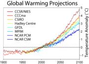
Coupled ocean-atmosphere GCMs use transient climate simulations to project/predict future temperature changes under various scenarios. These can be idealised scenarios (most commonly, CO2 increasing at 1%/yr) or more realistic (usually the "IS92a" or more recently the SRES scenarios). Which scenarios should be considered most realistic is currently uncertain, as the projections of future CO2 (and sulphate) emission are themselves uncertain.
The 2001 IPCC Third Assessment Report figure 9.3 shows the global mean response of 19 different coupled models to an idealised experiment in which CO2 is increased at 1% per year . Figure 9.5 shows the response of a smaller number of models to more realistic forcing. For the 7 climate models shown there, the temperature change to 2100 varies from 2 to 4.5 °C with a median of about 3 °C.
Future scenarios do not include unknowable events - for example, volcanic eruptions or changes in solar forcing. These effects are believed to be small in comparison to GHG forcing in the long term, but a large volcanic eruption, for example, could have a temporary cooling effect.
Human emissions of GHGs are an external input to the models, although it would be possible to couple in an economic model to provide these as well. Atmospheric GHG levels are usually supplied as an input, though it is possible to include a carbon cycle model including land vegetation and oceanic processes to calculate GHG levels.
Accuracy of models that predict global warming
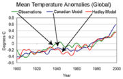
According to the IPCC, the majority of climatologists agree that important climate processes are imperfectly accounted for by the climate models but don't think that better models would change the conclusion. Scientists point out that there are specific flaws in the models, such as albedo errors, and external factors not taken into consideration that could change the conclusion above. GCMs are capable of reproducing the general features of the observed global temperature over the past century .
A debate over how to reconcile climate model predictions that upper air (tropospheric) warming should be greater than surface warming, with observations some of which appeared to show otherwise now appears to have been resolved in favour of the models, following revisions to the data: see satellite temperature record.
The effects of clouds are a significant area of uncertainty in climate models. Clouds have competing effects on the climate. One of the roles that clouds play in climate is in cooling the surface by reflecting sunlight back into space; another is warming by increasing the amount of infrared radiation emitted from the atmosphere to the surface. In the 2001 IPCC report on climate change, the possible changes in cloud cover were highlighted as one of the dominant uncertainties in predicting future climate change; see also .
Thousands of climate researchers around the world use climate models to understand the climate system. There are thousands of papers published about model-based studies in peer-reviewed journals - and a part of this research is work improving the models. Improvement has been difficult but steady (most obviously, state of the art AOGCMs no longer require flux correction), and progress has sometimes led to discovering new uncertainties.
In 2000, a comparison between measurements and dozens of GCM simulations of ENSO-driven tropical precipitation, water vapor, temperature, and outgoing longwave radiation found similarity between measurements and simulation of most factors. However the simulated change in precipitation was about one-fourth less than what was observed. Errors in simulated precipitation imply errors in other processes, such as errors in the evaporation rate that provides moisture to create precipitation. The other possibility is that the satellite-based measurements are in error. Either indicates progress is required in order to monitor and predict such changes.
A more complete discussion of climate models is provided by the IPCC TAR chapter 8, Model Evaluation (2001).
- The model mean exhibits good agreement with observations.
- The individual models often exhibit worse agreement with observations.
- Many of the non-flux adjusted models suffered from unrealistic climate drift up to about 1°C/century in global mean surface temperature.
- The errors in model-mean surface air temperature rarely exceed 1 °C over the oceans and 5 °C over the continents; precipitation and sea level pressure errors are relatively greater but the magnitudes and patterns of these quantities are recognisably similar to observations.
- Surface air temperature is particularly well simulated, with nearly all models closely matching the observed magnitude of variance and exhibiting a correlation > 0.95 with the observations.
- Simulated variance of sea level pressure and precipitation is within ±25% of observed.
- All models have shortcomings in their simulations of the present day climate of the stratosphere, which might limit the accuracy of predictions of future climate change.
- There is a tendency for the models to show a global mean cold bias at all levels.
- There is a large scatter in the tropical temperatures.
- The polar night jets in most models are inclined poleward with height, in noticeable contrast to an equatorward inclination of the observed jet.
- There is a differing degree of separation in the models between the winter sub-tropical jet and the polar night jet.
- For nearly all models the r.m.s. error in zonal- and annual-mean surface air temperature is small compared with its natural variability.
- There are problems in simulating natural seasonal variability. ( 2000)
- In flux-adjusted models, seasonal variations are simulated to within 2 K of observed values over the oceans. The corresponding average over non-flux-adjusted models shows errors up to about 6 K in extensive ocean areas.
- Near-surface land temperature errors are substantial in the average over flux-adjusted models, which systematically underestimates (by about 5 K) temperature in areas of elevated terrain. The corresponding average over non-flux-adjusted models forms a similar error pattern (with somewhat increased amplitude) over land.
- In Southern Ocean mid-latitudes, the non-flux-adjusted models overestimate the magnitude of January-minus-July temperature differences by ~5 K due to an overestimate of summer (January) near-surface temperature. This error is common to five of the eight non-flux-adjusted models.
- Over Northern Hemisphere mid-latitude land areas, zonal mean differences between July and January temperatures simulated by the non-flux-adjusted models show a greater spread (positive and negative) about observed values than results from the flux-adjusted models.
- The ability of coupled GCMs to simulate a reasonable seasonal cycle is a necessary condition for confidence in their prediction of long-term climatic changes (such as global warming), but it is not a sufficient condition unless the seasonal cycle and long-term changes involve similar climatic processes.
- There are problems in simulating natural seasonal variability. ( 2000)
- Coupled climate models do not simulate with reasonable accuracy clouds and some related hydrological processes (in particular those involving upper tropospheric humidity). Problems in the simulation of clouds and upper tropospheric humidity, remain worrisome because the associated processes account for most of the uncertainty in climate model simulations of anthropogenic change.
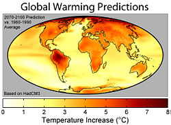
The precise magnitude of future changes in climate is still uncertain ; for the end of the 21st century (2071 to 2100), for SRES scenario A2, the change of global average SAT change from AOGCMs compared with 1961 to 1990 is +3.0 °C (4.8 °F) and the range is +1.3 to +4.5 °C (+2 to +7.2 °F).
Forecasts of climate change are inevitably uncertain. Even the degree of uncertainty is uncertain, a problem that stems from the fact that these climate models do not necessarily span the full range of known climate system behaviour.
Relation to weather forecasting
The global climate models used for climate projections are very similar in structure to (and often share computer code with) numerical models for weather prediction but are nonetheless logically distinct: see climate vs weather for details.
Most weather forecasting is done on the basis of interpreting the output of numerical model results. Since forecasts are short—typically a few days or a week—such models do not usually contain an ocean model but rely on imposed SSTs. They also require accurate initial conditions to begin the forecast—typically these are taken from the output of a previous forecast, with observations blended in. Because the results are needed quickly the predictions must be run in a few hours; but because they only need to cover a week of real time these predictions can be run at higher resolution than in climate mode. Currently the ECMWF runs at 40 km resolution as opposed to the 100-200 km scale used by typical climate models. Often nested models are run forced by the global models for boundary conditions, to achieve higher local resolution: for example, the Met Office runs a mesoscale model with an 11 km resolution covering the UK, and various agencies in the U.S. also run nested models such as the NGM and NAM models. Like most global numerical weather prediction models such as the GFS, global climate models are often spectral models instead of grid models. Spectral models are often used for global models because some computations in modeling can be performed faster thus reducing the time needed to run the model simulation.
