Image:Parabolic trajectory.svg
From Wikipedia, the free encyclopedia
Parabolic_trajectory.svg (SVG file, nominally 641 × 265 pixels, file size: 8 KB)
| |
This is a file from the Wikimedia Commons. The description on its description page there is shown below. |
| Description |
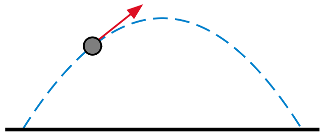
Illustration of a parabolic trajectory. |
|---|---|
| Source |
self-made with MATLAB. Tweaked in Inkscape. |
| Date |
05:58, 20 December 2007 (UTC) |
| Author |
Oleg Alexandrov |
| Permission ( Reusing this image) |
See below
|
 |
I, the copyright holder of this work, hereby release it into the public domain. This applies worldwide. In case this is not legally possible: Afrikaans | Alemannisch | Aragonés | العربية | Asturianu | Български | Català | Cebuano | Česky | Cymraeg | Dansk | Deutsch | Eʋegbe | Ελληνικά | English | Español | Esperanto | Euskara | Estremeñu | فارسی | Français | Galego | 한국어 | हिन्दी | Hrvatski | Ido | Bahasa Indonesia | Íslenska | Italiano | עברית | Kurdî / كوردی | Latina | Lietuvių | Latviešu | Magyar | Македонски | Bahasa Melayu | Nederlands | Norsk (bokmål) | Norsk (nynorsk) | 日本語 | Polski | Português | Ripoarisch | Română | Русский | Shqip | Slovenčina | Slovenščina | Српски / Srpski | Suomi | Svenska | ไทย | Tagalog | Türkçe | Українська | Tiếng Việt | Walon | 中文(简体) | 中文(繁體) | zh-yue-hant | +/- |
Source code ( MATLAB)
% illustration of a parabolic trajectory

function main()

   L=0.8;
   s=0.1;
   q=-0.4;
   N=100;

   arrow_size = 0.1;
   sharpness = 20;
   arrow_type = 1;
   arrlen = 0.3; % arrow length
   tiny = 0.01;
   ball_radius = 0.05;

   X=linspace(-L, L, N);
   Y =L^2 - X.^2;
   Xl = linspace(-L-s, L+s, N);


% KSmrq's colors
   red    = [0.867 0.06 0.14];
   blue   = [0, 129, 205]/256;
   green  = [0, 200,  70]/256;
   yellow = [254, 194,   0]/256;
   white = 0.99*[1, 1, 1];
   black = [0, 0, 0];
   gray = 0.5*white;
   lw = 2.3;


   figure(1); clf; hold on; axis equal; axis off;
   plot(X, Y, 'linewidth', lw, 'linestyle', '--', 'colour', blue);
   arrow([q-tiny, L^2-q^2], [q+arrlen-tiny, L^2-q^2-2*q*arrlen], lw, arrow_size, sharpness, arrow_type, red);
   ball(q, L^2 - q^2, ball_radius, gray)
   plot(Xl, 0*Xl, 'linewidth', 2*lw, 'colour', black);


  %saveas(gcf, 'Parabolic_trajectory.eps', 'psc2')
  plot2svg('Parabolic_trajectory.svg');

function ball(x, y, radius, colour) % draw a ball of given uniform colour
   Theta=0:0.1:2*pi;
   X=radius*cos(Theta)+x;
   Y=radius*sin(Theta)+y;
   H=fill(X, Y, colour);
   set(H, 'EdgeColor', [0, 0, 0]);

function arrow(start, stop, thickness, arrow_size, sharpness, arrow_type, colour)

% Function arguments:
% start, stop:  start and end coordinates of arrow, vectors of size 2
% thickness:    thickness of arrow stick
% arrow_size:   the size of the two sides of the angle in this picture ->
% sharpness:    angle between the arrow stick and arrow side, in degrees
% arrow_type:   1 for filled arrow, otherwise the arrow will be just two segments
% color:        arrow colour, a vector of length three with values in [0, 1]

% convert to complex numbers
   i=sqrt(-1);
   start=start(1)+i*start(2); stop=stop(1)+i*stop(2);
   rotate_angle=exp(i*pi*sharpness/180);

% points making up the arrow tip (besides the "stop" point)
   point1 = stop - (arrow_size*rotate_angle)*(stop-start)/abs(stop-start);
   point2 = stop - (arrow_size/rotate_angle)*(stop-start)/abs(stop-start);

   if arrow_type==1 % filled arrow

      % plot the stick, but not till the end, looks bad
      t=0.5*arrow_size*cos(pi*sharpness/180)/abs(stop-start); stop1=t*start+(1-t)*stop;
      plot(real([start, stop1]), imag([start, stop1]), 'LineWidth', thickness, 'Colour', colour);

      % fill the arrow
      H=fill(real([stop, point1, point2]), imag([stop, point1, point2]), colour);
      set(H, 'EdgeColor', 'none')

   else % two-segment arrow
      plot(real([start, stop]), imag([start, stop]),   'LineWidth', thickness, 'Colour', colour);
      plot(real([stop, point1]), imag([stop, point1]), 'LineWidth', thickness, 'Colour', colour);
      plot(real([stop, point2]), imag([stop, point2]), 'LineWidth', thickness, 'Colour', colour);
   end
File history
Click on a date/time to view the file as it appeared at that time.
| Date/Time | Dimensions | User | Comment | |
|---|---|---|---|---|
| current | 05:58, 20 December 2007 | 641×265 (8 KB) | Oleg Alexandrov | ({{Information |Description=Illustration of a parabolic trajectory. |Source=self-made with MATLAB |Date=~~~~~ |Author= Oleg Alexandrov |Permission=See below |other_versions= }} {{PD-self}} ==Source code ( MATLAB)== ) |