Image:Newton iteration.png
From Wikipedia, the free encyclopedia
Size of this preview: 583 × 479 pixels
Full resolution (2,406 × 1,978 pixels, file size: 55 KB, MIME type: image/png)
| |
This is a file from the Wikimedia Commons. The description on its description page there is shown below. |
 A vector version of this image (SVG) is available. For more information about vector graphics, read about Commons transition to SVG. Deutsch | English | Español | Français | Galego | עברית | Magyar | Italiano | 日本語 | 한국어 | Lietuvių | Polski | Português | Русский | Српски / Srpski | Українська | +/- |
 |
| Description |
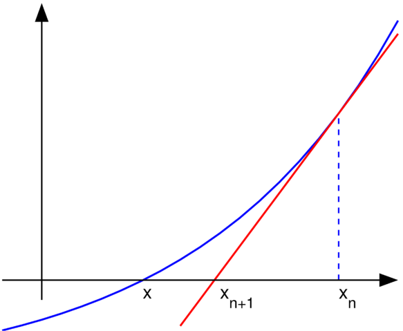
Uploader graphed this with en:MATLAB (Illustration of en:Newton's method) |
|---|---|
| Source |
Originally from en.wikipedia; description page is/was here. |
| Date |
2004-11-22 (first version); 2004-11-23 (last version) |
| Author |
Original uploader was Olegalexandrov at en.wikipedia |
| Permission ( Reusing this image) |
Released into the public domain (by the author).
|
Source code
% illustration of Newton's method for finding a zero of a function

function main ()

a=-1; b=1;   % interval endpoints
fs=20;       % text font size

% arrows settings
thickness1=2; thickness2=1.5; arrowsize=0.1; arrow_type=1;
angle=20; % in degrees

h=0.1;  % grid size
X=a:h:b; % points on the x axis
f=inline('exp(x)/1.5-0.5');   % function to plot
g=inline('exp(x)/1.5');       % derivative of f
x0=0.7; y0=f(x0);             % point at which to draw the tangent line
m=g(x0);
Y=f(X);                       % points on the function to plot
XT=-0.1:h:b; YT=y0+(XT-x0)*m; % tangent line

% prepare the screen
clf; hold on; axis equal; axis off

% plot the graph and the tangent lines
plot(X, Y, 'linewidth', thickness1)
plot(XT, YT, 'r', 'linewidth', thickness1)
plot([x0 x0], [0, y0], '--', 'linewidth', thickness2)

% axes
small=0.2;
arrow([a 0], [b, 0], thickness2, arrowsize, angle, arrow_type, [0, 0, 0])
arrow([a+small, -0.1], [a+small, 1.4], thickness2, arrowsize, angle, arrow_type, [0, 0, 0])

% text
H=text(-0.29, -0.06,  'x'); set(H, 'fontsize', fs)
H=text(0.1, -0.1,  'x_{n+1}'); set(H, 'fontsize', fs)
H=text(0.7, -0.1,  'x_{n}'); set(H, 'fontsize', fs)

% save to disk
saveas(gcf, 'newton_iteration.eps', 'psc2')

function arrow(start, stop, thickness, arrow_size, sharpness, arrow_type, color)

% Function arguments:
% start, stop:  start and end coordinates of arrow, vectors of size 2
% thickness:    thickness of arrow stick
% arrow_size:   the size of the two sides of the angle in this picture ->
% sharpness:    angle between the arrow stick and arrow side, in degrees
% arrow_type:   1 for filled arrow, otherwise the arrow will be just two segments
% color:        arrow color, a vector of length three with values in [0, 1]

% convert to complex numbers
   i=sqrt(-1);
   start=start(1)+i*start(2); stop=stop(1)+i*stop(2);
   rotate_angle=exp(i*pi*sharpness/180);

% points making up the arrow tip (besides the "stop" point)
   point1 = stop - (arrow_size*rotate_angle)*(stop-start)/abs(stop-start);
   point2 = stop - (arrow_size/rotate_angle)*(stop-start)/abs(stop-start);

   if arrow_type==1 % filled arrow

      % plot the stick, but not till the end, looks bad
      t=0.5*arrow_size*cos(pi*sharpness/180)/abs(stop-start); stop1=t*start+(1-t)*stop;
      plot(real([start, stop1]), imag([start, stop1]), 'LineWidth', thickness, 'Color', color);

      % fill the arrow
      H=fill(real([stop, point1, point2]), imag([stop, point1, point2]), color);
      set(H, 'EdgeColor', 'none')

   else % two-segment arrow
      plot(real([start, stop]), imag([start, stop]),   'LineWidth', thickness, 'Color', color);
      plot(real([stop, point1]), imag([stop, point1]), 'LineWidth', thickness, 'Color', color);
      plot(real([stop, point2]), imag([stop, point2]), 'LineWidth', thickness, 'Color', colour);
   end
License information
 |
This image has been (or is hereby) released into the public domain by its author, Olegalexandrov at the English Wikipedia project. This applies worldwide. In case this is not legally possible: |
Original upload log
(All user names refer to en.wikipedia)
- 2004-11-23 19:55 Olegalexandrov 405×340×8 (14290 bytes) Scaled down the picture of Newton's method
- 2004-11-22 21:34 Olegalexandrov 509×406×8 (16510 bytes) I graphed this with Matlab (Illustration of Newton's method) {{PD}}
File history
Click on a date/time to view the file as it appeared at that time.
| Date/Time | Dimensions | User | Comment | |
|---|---|---|---|---|
| current | 03:23, 25 May 2007 | 2,406×1,978 (55 KB) | Oleg Alexandrov | ({{Information |Description=Uploader graphed this with en:MATLAB (Illustration of en:Newton's method) ==Source code== <pre> <nowiki> % illustration of Newton's method for finding a zero of a function function main () a=-1; b=1; % interva) |
| 23:11, 12 June 2005 | 405×340 (6 KB) | Everlong | (optimized for smaller file size) | |
| 23:06, 17 January 2005 | 405×340 (14 KB) | Andreas Ipp | ({{PD}}: Original author graphed this with MATLAB (Illustration of Newton's method), from Wikipedia.) |