Inductance
2008/9 Schools Wikipedia Selection. Related subjects: Electricity and Electronics
| Electromagnetism | ||||||||||||
 |
||||||||||||
Electricity · Magnetism
|
||||||||||||
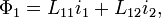
An electric current i flowing around a circuit produces a magnetic field and hence a magnetic flux Φ through the circuit. The ratio of the magnetic flux to the current is called the inductance, or more accurately self-inductance of the circuit. The term was coined by Oliver Heaviside in February 1886. It is customary to use the symbol L for inductance, possibly in honour of the physicist Heinrich Lenz. The quantitative definition of the inductance per coil turn in SI units ( webers per ampere) is

In honour of Joseph Henry, the unit of inductance has been given the name henry (H): 1H = 1Wb/A.
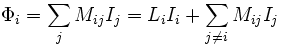
In the above definition, the magnetic flux Φ is that caused by the current flowing through the circuit concerned. There may, however, be contributions from other circuits. Consider for example two circuits C1, C2, carrying the currents i1, i2. The magnetic fluxes Φ1 and Φ2 in C1 and C2, respectively, are given by
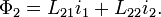
According to the above definition, L11 and L22 are the self-inductances of C1 and C2, respectively. It can be shown (see below) that the other two coefficients are equal: L12 = L21 = M, where M is called the mutual inductance of the pair of circuits.
Self and mutual inductances also occur in the expression
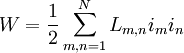
for the energy of the magnetic field generated by N electrical circuits carrying the currents in. This equation is an alternative definition of inductance, also valid when the currents don't flow in thin wires and when it thus is not immediately clear what the area encompassed by a circuit is and how the magnetic flux through the circuit is to be defined. The definition L = Φ / i, in contrast, is more direct and more intuitive. It may be shown that the two definitions are equivalent by equating the time derivate of W and the electric power transferred to the system.
Properties of inductance
The equation relating inductance and flux linkages can be rearranged as follows:

Taking the time derivative of both sides of the equation yields:
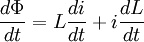
In most physical cases, the inductance is constant with time and so

By Faraday's Law of Induction we have:
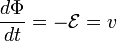
where  is the Electromotive force (emf) and v is the induced voltage. Note that the emf is opposite to the induced voltage. Thus:

or
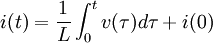
These equations together state that, for a steady applied voltage v, the current changes in a linear manner, at a rate proportional to the applied voltage, but inversely proportional to the inductance. Conversely, if the current through the inductor is changing at a constant rate, the induced voltage is constant.
The effect of inductance can be understood using a single loop of wire as an example. If a voltage is suddenly applied between the ends of the loop of wire, the current must change from zero to non-zero. However, a non-zero current induces a magnetic field by Ampère's law. This change in the magnetic field induces an emf that is in the opposite direction of the change in current. The strength of this emf is proportional to the change in current and the inductance. When these opposing forces are in balance, the result is a current that increases linearly with time where the rate of this change is determined by the applied voltage and the inductance.
Multiplying the equation for di / dt above with Li leads to
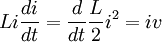
Since iv is the energy transferred to the system per time it follows that  is the energy of the magnetic field generated by the current.
Phasor circuit analysis and impedance
Using phasors, the equivalent impedance of an inductance is given by:
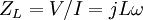
where
- j is the imaginary unit,
- L is the inductance,
 is the angular frequency,
- f is the frequency and
 is the inductive reactance.
 - L is the inductance,
Induced emf
The flux  through the i-th circuit in a set is given by:
so that the induced emf, , of a specific circuit, i, in any given set can be given directly by:

Coupled inductors

Mutual inductance is the concept that the change in current in one inductor can induce a voltage in another nearby inductor. It is important as the mechanism by which transformers work, but it can also cause unwanted coupling between conductors in a circuit.
The mutual inductance, M, is also a measure of the coupling between two inductors. The mutual inductance by circuit i on circuit j is given by the double integral Neumann formula, see #Calculation techniques
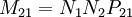
The mutual inductance also has the relationship:
where
- M21 is the mutual inductance, and the subscript specifies the relationship of the voltage induced in coil 2 to the current in coil 1.
- N1 is the number of turns in coil 1,
- N2 is the number of turns in coil 2,
- P21 is the permeance of the space occupied by the flux.
- N1 is the number of turns in coil 1,
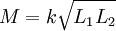
The mutual inductance also has a relationship with the coupling coefficient. The coupling coefficient is always between 1 and 0, and is a convenient way to specify the relationship between a certain orientation of inductor with arbitrary inductance:
where
- k is the coupling coefficient and 0 ≤ k ≤ 1,
- L1 is the inductance of the first coil, and
- L2 is the inductance of the second coil.
- L1 is the inductance of the first coil, and
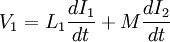
Once this mutual inductance factor M is determined, it can be used to predict the behaviour of a circuit:
where
- V is the voltage across the inductor of interest,
- L1 is the inductance of the inductor of interest,
- dI1 / dt is the derivative, with respect to time, of the current through the inductor of interest,
- M is the mutual inductance and
- dI2 / dt is the derivative, with respect to time, of the current through the inductor that is coupled to the first inductor.
- L1 is the inductance of the inductor of interest,
When one inductor is closely coupled to another inductor through mutual inductance, such as in a transformer, the voltages, currents, and number of turns can be related in the following way:

where
- Vs is the voltage across the secondary inductor,
- Vp is the voltage across the primary inductor (the one connected to a power source),
- Ns is the number of turns in the secondary inductor, and
- Np is the number of turns in the primary inductor.
- Vp is the voltage across the primary inductor (the one connected to a power source),
Conversely the current:

where
- Is is the current through the secondary inductor,
- Ip is the current through the primary inductor (the one connected to a power source),
- Ns is the number of turns in the secondary inductor, and
- Np is the number of turns in the primary inductor.
- Ip is the current through the primary inductor (the one connected to a power source),
Note that the power through one inductor is the same as the power through the other. Also note that these equations don't work if both transformers are forced (with power sources).
When either side of the transformer is a tuned circuit, the amount of mutual inductance between the two windings determines the shape of the frequency response curve. Although no boundaries are defined, this is often referred to as loose-, critical-, and over-coupling. When two tuned circuits are loosely coupled through mutual inductance, the bandwidth will be narrow. As the amount of mutual inductance increases, the bandwidth continues to grow. When the mutual inductance is increased beyond a critical point, the peak in the response curve begins to drop, and the centre frequency will be attenuated more strongly than its direct sidebands. This is known as overcoupling.
Calculation techniques
Mutual inductance
The mutual inductance by circuit i on circuit j is given by the double integral Neumann formula
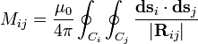
The constant μ0 is the permeability of free space (4π × 10-7 H/m), Ci and Cj are the curves spanned by the wires, Rij is the distance between two points. See a derivation of this equation.
Self-inductance
Formally the self-inductance of a wire loop would be given by the above equation with i =j. However, 1 / R now gets singular and the finite radius a and the distribution of the current in the wire must be taken into account. There remain the contribution from the integral over all points where  and a correction term,
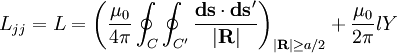
Here a and l denote radius and length of the wire, and Y is a constant that depends on the distribution of the current in the wire: Y = 0 when the current flows in the surface of the wire ( skin effect), Y = 1 / 4 when the current is homogenuous across the wire. Here is a derivation of this equation.
Self-inductance of simple electrical circuits
The self-inductance of many types of electrical circuits can be given in closed form. Examples are listed in the table.
| Type | Inductance / μ0 | Comment |
|---|---|---|
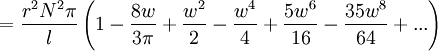
| Single layer solenoid |

|
N: Number of turns r: Radius l: Length w = r / l m = 4w2 E,K: Elliptic integrals |
| Coaxial cable, high frequency |
 |
a1: Outer radius a: Inner radius l: Length |
| Circular loop | 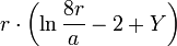 |
r: Loop radius a: Wire radius |
| Rectangle |  |
b, d: Border length d >> a, b >> a a: Wire radius |
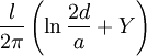
| Pair of parallel wires |
 |
a: Wire radius d: Distance, d ≥ 2a l: Length of pair |
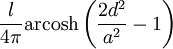
| Pair of parallel wires, high frequency |
 |
a: Wire radius d: Distance, d ≥ 2a l: Length of pair |
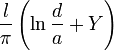
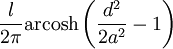
| Wire parallel to conducting wall |
 |
a: Wire radius d: Distance, d ≥ a l: Length |
| Wire parallel to conducting wall, high frequency |
 |
a: Wire radius d: Distance, d ≥ a l: Length |
The constant μ0 is the permeability of free space (4π × 10-7 H/m). For high frequencies the electrical current flows in the conductor surface ( skin effect), and depending on the geometry it sometimes is necessary to distinguish low and high frequency inductances. This is the purpose of the constant Y: Y=0 when the current is uniformly distributed over the surface of the wire (skin effect), Y=1/4 when the current is uniformly distributed over the cross section of the wire. In the high frequency case, if conductors approach each other, an additional screening current flows in their surface, and expressions containing Y become invalid.
Inductance of a solenoid
A solenoid is a long, thin coil, i.e. a coil whose length is much greater than the diameter. Under these conditions, and without any magnetic material used, the magnetic flux density B within the coil is practically constant and is given by
where μ0 is the permeability of free space, N the number of turns, i the current and l the length of the coil. Ignoring end effects the total magnetic flux through the coil is obtained by multiplying the flux density B by the cross-section area A and the number of turns N:
from which it follows that the inductance of a solenoid is given by:
This, and the inductance of more complicated shapes, can be derived from Maxwell's equations. For rigid air-core coils, inductance is a function of coil geometry and number of turns, and is independent of current.
Similar analysis applies to a solenoid with a magnetic core, but only if the length of the coil is much greater than the product of the relative permeability of the magnetic core and the diameter. That limits the simple analysis to low-permeability cores, or extremely long thin solenoids. Although rarely useful, the equations are,
where μr the relative permeability of the material within the solenoid,
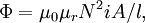
from which it follows that the inductance of a solenoid is given by:
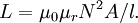
Note that since the permeability of ferromagnetic materials changes with applied magnetic flux, the inductance of a coil with a ferromagnetic core will generally vary with current.
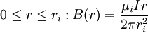
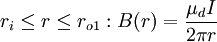
Inductance of a coaxial line
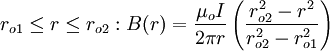
Let the inner conductor have radius ri and permeability μi, let the dielectric between the inner and outer conductor have permeability μd, and let the outer conductor have inner radius ro1, outer radius ro2, and permeability μo. Assume that a DC current I flows in opposite directions in the two conductors, with uniform current density. The magnetic field generated by these currents points in the azimuthal direction and is a function of radius r; it can be computed using Ampère's Law:
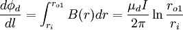
The flux per length l in the region between the conductors can be computed by drawing a surface containing the axis:
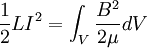
Inside the conductors, L can be computed by equating the energy stored in an inductor,  , with the energy stored in the magnetic field:
For a cylindrical geometry with no l dependence, the energy per unit length is
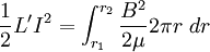
where L' is the inductance per unit length. For the inner conductor, the integral on the right-hand-side is  ; for the outer conductor it is
Solving for L' and summing the terms for each region together gives a total inductance per unit length of:

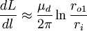
However, for a typical coaxial line application we are interested in passing (non-DC) signals at frequencies for which the resistive skin effect cannot be neglected. In most cases, the inner and outer conductor terms are negligible, in which case one may approximate
Links
- Clemson Vehicular Electronics Laboratory: Inductance Calculator