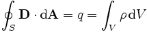
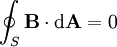
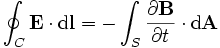
Maxwell's equations
2008/9 Schools Wikipedia Selection. Related subjects: Electricity and Electronics
| Electromagnetism | ||||||||||||
 |
||||||||||||
Electricity · Magnetism
|
||||||||||||
In electromagnetism, Maxwell's equations are a set of equations first presented as a distinct group in the later half of the nineteenth century by James Clerk Maxwell. They describe the interrelationship between electric fields, magnetic fields, electric charge, and electric current.
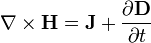
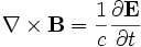
Although Maxwell himself was not the originator of the individual equations, he derived them again independently in conjunction with his molecular vortex model of Faraday's lines of force, and he was the person who first grouped these equations all together into a coherent set. Most importantly, he introduced an extra term to Ampère's Circuital Law. This extra term is the time derivative of electric field and is known as Maxwell's displacement current. Maxwell's modified version of Ampère's Circuital Law enables the set of equations to be combined together to derive the electromagnetic wave equation.
Although Maxwell's equations were known before special relativity, they can be derived from Coulomb's law and special relativity if one assumes invariance of electric charge.
History of Maxwell's Equations
Maxwell's equations are a set of four equations that can all be found at various places in Maxwell's 1861 paper On Physical Lines of Force. They express (i) how electric charges produce electric fields ( Gauss's law), (ii) the experimental absence of magnetic monopoles, (iii) how electric currents and changing electric fields produce magnetic fields ( Ampère's Circuital Law), and (iv) how changing magnetic fields produce electric fields ( Faraday's law of induction).
Apart from Maxwell's amendment to Ampère's Circuital Law, none of these equations are original. However, Maxwell uniquely re-derived them hydrodynamically and mechanically using his vortex model of Faraday's lines of force.
In the year 1884 Oliver Heaviside selected these four equations, and in conjunction with Willard Gibbs, he put them into modern vector notation. This gives rise to the claim by some scientists that Maxwell's equations are in actual fact Heaviside's equations.
This matter is further confused by the fact that the term 'Maxwell's Equations' is also used to describe a set of eight equations labelled (A) to (H) in Maxwell's 1865 paper A Dynamical Theory of the Electromagnetic Field. It therefore helps when referring to 'Maxwell's Equations' to specify whether we are talking about the original eight equations or the modified 'Heaviside Four'.
The two sets of equations are physically equivalent to all intents and purposes although Gauss's Law is the only actual equation that appears in both sets. The Lorentz force that appears as equation (D) in the original eight is the solution to Faraday's law of electromagnetic induction that appears in the 'Heaviside Four', and the Maxwell/Ampère equation in the 'Heaviside Four' is an amalgamation of two equations in the original eight.
Summary of the Modern Heaviside Versions
Symbols in bold represent vector quantities, whereas symbols in italics represent scalar quantities.
General case
| Name | Differential form | Integral form |
|---|---|---|
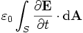
| Gauss's law: |  |
 |
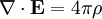
| Gauss' law for magnetism (absence of magnetic monopoles): |
 |
 |
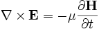
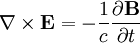
| Faraday's law of induction: | 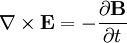 |
 |
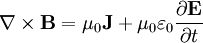
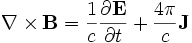
| Ampère's Circuital Law (with Maxwell's extension): |
 |
 |
The following table provides the meaning of each symbol and the SI unit of measure:
| Symbol | Meaning | SI Unit of Measure |
|---|---|---|
 |
electric field | volt per meter or, equivalently, newton per coulomb |
| μ | magnetic permeability of the medium | henries per meter, or newtons per ampere squared |
| iN | net electrical current enclosed by an Amperian line | amperes |
| q | net electric charge enclosed by the Gaussian surface | coulombs |
 |
magnetic field also called the auxiliary field |
ampere per meter |
 |
electric displacement field also called the electric flux density |
coulomb per square meter |
 |
magnetic flux density also called the magnetic induction also called the magnetic field |
tesla, or equivalently, weber per square meter |
 |
free electric charge density, not including dipole charges bound in a material |
coulomb per cubic meter |
 |
free current density, not including polarization or magnetization currents bound in a material |
ampere per square meter |
 |
differential vector element of surface area A, with infinitesimally small magnitude and direction normal to surface S |
square meters |
 |
differential element of volume V enclosed by surface S | cubic meters |
 |
differential vector element of path length tangential to contour C enclosing surface S | meters |
 |
the divergence operator | per meter |
 |
the curl operator | per meter |
Although SI units are given here for the various symbols, Maxwell's equations are unchanged in many systems of units (and require only minor modifications in all others). The most commonly used systems of units are SI, used for engineering, electronics and most practical physics experiments, and Planck units (also known as "natural units"), used in theoretical physics, quantum physics and cosmology. An older system of units, the cgs system, is also used.
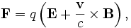
In order to complete the theory of electromagnetism we need to add another equation to Heaviside's group of four 'Maxwell's Equations'. The force exerted upon a charged particle by the electric field and magnetic field is given by the Lorentz force equation:
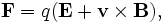
where  is the charge on the particle and
  is the particle velocity. This is slightly different when expressed in the cgs system of units below.
This extra equation appeared in cartesian format as equation (D) of the original eight 'Maxwell's Equations'.
Maxwell's equations are generally applied to macroscopic averages of the fields, which vary wildly on a microscopic scale in the vicinity of individual atoms (where they undergo quantum mechanical effects as well). It is only in this averaged sense that one can define quantities such as the permittivity and permeability of a material, below (the microscopic Maxwell's equations, ignoring quantum effects, are simply those of a vacuum — but one must include all atomic charges and so on, which is generally an intractable problem).
In linear materials
In linear materials, the polarization density  (in coulombs per square meter) and magnetization density
  (in amperes per meter) are given by:


and the and fields are related to and by:


where:
χe is the electrical susceptibility of the material,
χm is the magnetic susceptibility of the material,
 is the electrical permittivity of the material, and
μ is the magnetic permeability of the material
(This can actually be extended to handle nonlinear materials as well, by making ε and μ depend upon the field strength; see e.g. the Kerr and Pockels effects.)
In non-dispersive, isotropic media, ε and μ are time-independent scalars, and Maxwell's equations reduce to

In a uniform (homogeneous) medium, ε and μ are constants independent of position, and can thus be furthermore interchanged with the spatial derivatives.
More generally, ε and μ can be rank-2 tensors (3×3 matrices) describing birefringent (anisotropic) materials. Also, although for many purposes the time/frequency-dependence of these constants can be neglected, every real material exhibits some material dispersion by which ε and/or μ depend upon frequency (and causality constrains this dependence to obey the Kramers-Kronig relations).
In vacuum, without charges or currents
The vacuum is a linear, homogeneous, isotropic, dispersionless medium, and the proportionality constants in the vacuum are denoted by ε0 and μ0 (neglecting very slight nonlinearities due to quantum effects).


Since there is no current or electric charge present in the vacuum, we obtain the Maxwell equations in free space:


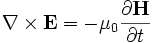
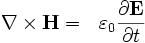
These equations have a solution in terms of travelling sinusoidal plane waves, with the electric and magnetic field directions orthogonal to one another and the direction of travel, and with the two fields in phase, travelling at the speed

Maxwell discovered that this quantity c is simply the speed of light in vacuum, and thus that light is a form of electromagnetic radiation. The currently accepted values for the speed of light, the permittivity, and the permeability are summarized in the following table:
| Symbol | Name | Numerical Value | SI Unit of Measure | Type |
|---|---|---|---|---|
 |
Speed of light |  |
meters per second | defined |
 |
Permittivity |  |
farads per meter | derived |
 |
Permeability |  |
henries per meter | defined |
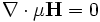
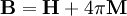
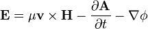
The Difference between the Magnetic Induction Vector B and the Magnetic Field Vector H
The difference between the vector and the vector can be traced back to Maxwell's 1855 paper entitled 'On Faraday's Lines of Force'. It is later clarified in his concept of a sea of molecular vortices that appears in his 1861 paper On Physical Lines of Force - 1861. Within that context, represented pure vorticity (spin), whereas was a weighted vorticity that was weighted for the density of the vortex sea. Maxwell considered magnetic permeability μ to be a measure of the density of the vortex sea. Hence the relationship,
(1) Magnetic Induction Current

was essentially a rotational analogy to the linear electric current relationship,
(2) Electric Convection Current

where ρ is electric charge density and v is movement. was seen as a kind of magnetic current of vortices aligned in their axial planes, with being the circumferential velocity of the vortices.
The electric current equation can be viewed as a convective current of electric charge that involves linear motion. By analogy, the magnetic equation is an inductive current involving spin. There is no linear motion in the inductive current along the direction of the vector. The magnetic inductive current represents lines of force. In particular, it represents lines of inverse square law force.
The extension of the above considerations confirms that where is to , and where is to ρ, then it necessarily follows from Gauss's law and from the equation of continuity of charge that is to . Ie. parallels with , whereas parallels with .
The Heaviside Versions in Detail
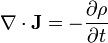
(1) Gauss's Law
Gauss's law yields the sources (and sinks) of electric charge.
where ρ is the free electric charge density (in units of C/m3), not including dipole charges bound in a material, and is the electric displacement field (in units of C/m2). The solution to Gauss's Law is Coulomb's law for stationary charges in vacuum.
The equivalent integral form (by the divergence theorem), also known as Gauss' law, is:
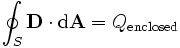
where is the area of a differential square on the closed surface A with an outward facing surface normal defining its direction, and Qenclosed is the free charge enclosed by the surface.
In a linear material, is directly related to the electric field via a material-dependent constant called the permittivity, ε:
 .
.
Any material can be treated as linear, as long as the electric field is not extremely strong. The permittivity of free space is referred to as ε0, and appears in:

where, again, is the electric field (in units of V/m), ρt is the total charge density (including bound charges), and ε0 (approximately 8.854 pF/m) is the permittivity of free space. ε can also be written as  , where εr is the material's relative permittivity or its dielectric constant.
Compare Poisson's equation.
(2) The Divergence of the Magnetic Field
The divergence of a magnetic field is always zero and hence magnetic field lines are solenoidal.
is the magnetic flux density (in units of teslas, T), also called the magnetic induction.
Equivalent integral form:
is the area of a differential square on the surface A with an outward facing surface normal defining its direction.
Like the electric field's integral form, this equation only works if the integral is done over a closed surface.
This equation is related to the magnetic field's structure because it states that given any volume element, the net magnitude of the vector components that point outward from the surface must be equal to the net magnitude of the vector components that point inward. Structurally, this means that the magnetic field lines must be closed loops. Another way of putting it is that the field lines cannot originate from somewhere; attempting to follow the lines backwards to their source or forward to their terminus ultimately leads back to the starting position. Hence, this is a mathematical formulation of the statement that there are no magnetic monopoles.
(3) Faraday's Law of Electromagnetic Induction
The equivalent integral form is:
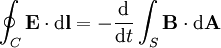
where
 is the electric field,
 is the boundary of the surface S.
If a conducting wire, following the contour C, is introduced into the field the so-called electromotive force in this wire is equal to the value of these integrals (over the fields in absence of the wire!).
The negative sign is necessary to maintain conservation of energy. It is so important that it even has its own name, Lenz's law.
This equation relates the electric and magnetic fields, but it also has a number of practical applications. This equation describes how electric motors and electric generators work. Specifically, it demonstrates that a voltage can be generated by varying the magnetic flux passing through a given area over time, such as by uniformly rotating a loop of wire through a fixed magnetic field. In a motor or generator, the fixed excitation is provided by the field circuit and the varying voltage is measured across the armature circuit. In some types of motors/generators, the field circuit is mounted on the rotor and the armature circuit is mounted on the stator, but other types of motors/generators reverse the configuration.
Maxwell's equations apply to a right-handed coordinate system. To apply them unmodified to a left handed system would reverse the polarity of magnetic fields (not inconsistent, but confusingly against convention).
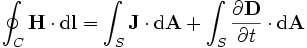
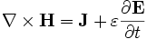
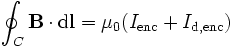
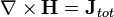
(4) Ampère's Circuital Law
Ampère's Circuital Law describes the source of the magnetic field,
where is the magnetic field strength (in units of A/m), related to the magnetic flux by a constant called the permeability, μ (), and is the current density, defined by:  where
where  is a vector field called the drift velocity that describes the velocities of the charge carriers which have a density described by the scalar function ρq. The second term on the right hand side of Ampère's Circuital Law is known as the displacement current.
It was Maxwell who added the displacement current term to Ampère's Circuital Law at equation (112) in his 1861 paper On Physical Lines of Force. This addition means that either Maxwell's original eight equations, or the modified Heaviside four equations can be combined together to obtain the electromagnetic wave equation.
Maxwell used the displacement current in conjunction with the original eight equations in his 1864 paper A Dynamical Theory of the Electromagnetic Field to derive the electromagnetic wave equation in a much more cumbersome fashion that that which is employed when using the 'Heaviside Four'. Most modern textbooks derive the electromagnetic wave equation using the 'Heaviside Four'.
In free space, the permeability μ is the permeability of free space, μ0, which is defined to be exactly 4π×10-7 Wb/A•m. Also, the permittivity becomes the permittivity of free space ε0. Thus, in free space, the equation becomes:
Equivalent integral form:
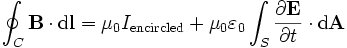
 is the edge of the open surface A (any surface with the curve as its edge will do), and Iencircled is the current encircled by the curve (the current through any surface is defined by the equation:
 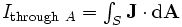 ). In some situations, this integral form of Ampere-Maxwell Law appears in:
for
is sometimes called displacement current
If the electric flux density does not vary rapidly, the second term on the right hand side (the displacement flux) is negligible, and the equation reduces to Ampere's law.
Maxwell's equations in CGS units
The above equations are given in the International System of Units, or SI for short. In a related unit system, called cgs (short for centimeter-gram-second), the equations take the following form:
Where c is the speed of light in a vacuum. For the electromagnetic field in a vacuum, the equations become:
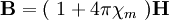
In this system of units the relation between magnetic induction, magnetic field and total magnetization take the form:
With the linear approximation:
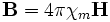
χm for vacuum is zero and therefore:

and in the ferro or ferri magnetic materials where χm is much bigger than 1:
The force exerted upon a charged particle by the electric field and magnetic field is given by the Lorentz force equation:
where is the charge on the particle and is the particle velocity. This is slightly different from the SI-unit expression above. For example, here the magnetic field  has the same units as the electric field
  .
.
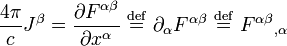
Formulation of Maxwell's equations in special relativity
In special relativity, in order to more clearly express the fact that Maxwell's equations (in vacuum) take the same form in any inertial coordinate system, the vacuum Maxwell's equations are written in terms of four-vectors and tensors in the "manifestly covariant" form (cgs units):
 ,
,
and

where  is the 4-current,
  is the field strength tensor,
  is the Levi-Civita symbol, and
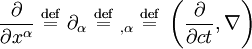
is the 4-gradient. Repeated indices are summed over according to Einstein summation convention. We have displayed the results in several common notations.
The first tensor equation is an expression of the two inhomogeneous Maxwell's equations, Gauss' law and Ampere's law with Maxwell's correction. The second equation is an expression of the homogenous equations, Faraday's law of induction and the absence of magnetic monopoles.
Maxwell's equations in terms of differential forms
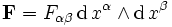
In a vacuum, where ε and μ are constant everywhere, Maxwell's equations simplify considerably once the language of differential geometry and differential forms is used. The electric and magnetic fields are now jointly described by a 2-form F in a 4-dimensional spacetime manifold. Maxwell's equations then reduce to the Bianchi identity
where d denotes the exterior derivative - a differential operator acting on forms - and the source equation

where the (dual) Hodge star operator * is a linear transformation from the space of 2 forms to the space of 4-2 forms defined by the metric in Minkowski space (or in four dimensions by its conformal class), and the fields are in natural units where 1 / 4πε0 = 1. Here, the 3-form J is called the "electric current" or " current (3-)form" satisfying the continuity equation

As the exterior derivative is defined on any manifold, this formulation of electromagnetism works for any 4-dimensional oriented manifold with a Lorentz metric, e.g. on the curved space-time of general relativity.
In a linear, macroscopic theory, the influence of matter on the electromagnetic field is described through more general linear transformation in the space of 2-forms. We call

the constitutive transformation. The role of this transformation is comparable to the Hodge duality transformation. The Maxwell equations in the presence of matter then become:

where the current 3-form J still satisfies the continuity equation dJ= 0.
When the fields are expressed as linear combinations (of exterior products) of basis forms  ,
,
 .
.
the constitutive relation takes the form
where the field coefficient functions are antisymmetric in the indices and the constitutive coefficients are antisymmetric in the corresponding pairs. The Hodge duality transformation leading to the vacuum equations discussed above are obtained by taking
which up to scaling is the only invariant tensor of this type that can be defined with the metric.
In this formulation, electromagnetism generalises immediately to any 4 dimensional oriented manifold or with small adaptations any manifold, requiring not even a metric. Thus the expression of Maxwell's equations in terms of differential forms leads to a further notational simplification. Whereas Maxwell's Equations could be written as two tensor equations instead of eight scalar equations, from which the propagation of electromagnetic disturbances and the continuity equation could be derived with a little effort, using differential forms leads to an even simpler derivation of these results. The price one pays for this simplification, however, is a need for knowledge of more technical mathematics.
Conceptual insight from this formulation
On the conceptual side, from a point of view of physics, this shows that the second and third Maxwell equations should be grouped together, be called the homogeneous ones, and be seen as geometric identities expressing nothing else that the field F derives from a more "fundamental" potential A, while the first and last one should be seen as the dynamical equations of motion, obtained via the Lagrangian principle of least action, from the "interaction term" A J (introduced through gauge covariant derivatives), coupling the field to matter.
Often, the time derivative in the third law motivates calling this equation "dynamical", which is somewhat misleading; in the sense of the preceding analysis, this is rather an artifact of breaking relativistic covariance by choosing a preferred time direction. To have physical degrees of freedom propagated by these field equations, one must include a kinetic term F *F for A; and take into account the non-physical degrees of freedom which can be removed by gauge transformation A→A' = A-dα: see also gauge fixing and Fadeev-Popov ghosts.
The original eight Maxwell's Equations
In Part III of A Dynamical Theory of the Electromagnetic Field which is entitled "GENERAL EQUATIONS OF THE ELECTROMAGNETIC FIELD" (page 480 of the article and page 2 of the pdf link), Maxwell formulated eight equations labelled A to H. These eight equations were to become known as Maxwell's equations. Nowadays however, references to Maxwell's equations invariably refer to the Heaviside versions. Heaviside's versions of Maxwell's equations actually only contain one of the original eight, i.e. equation G Gauss's Law. Another of Heaviside's four equations is an amalgamation of Maxwell's Law of Total Currents (equation A) with Ampère's Circuital Law (equation C). This amalgamation, which Maxwell himself had actually originally made at equation (112) in his 1861 paper " On Physical Lines of Force", is the one that modifies Ampère's Circuital Law to include Maxwell's Displacement current.
The eight original Maxwell's equations will now be listed in modern vector notation,
(A) The Law of Total Currents
(B) Definition of the Magnetic Vector Potential
(C) Ampère's Circuital Law
(D) The Lorentz Force. Electric fields created by convection, induction, and by charges.
(E) The Electric Elasticity Equation

(F) Ohm's Law

(G) Gauss's Law
(H) Equation of Continuity of Charge
Notation
- is the magnetic field, which Maxwell called the "magnetic intensity". is the electric current density (with
 being the total current including displacement current). is the displacement field (called the "electric displacement" by Maxwell).
- ρ is the free charge density (called the "quantity of free electricity" by Maxwell).
 is the magnetic vector potential (called the "angular impulse" by Maxwell). is the electric field (called the "electromotive force" by Maxwell, not to be confused with the scalar quantity that is now called electromotive force).
- φ is the electric potential (which Maxwell also called "electric potential").
- σ is the electrical conductivity (Maxwell called the inverse of conductivity the "specific resistance", what is now called the resistivity).
Maxwell did not consider completely general materials; his initial formulation used linear, isotropic, nondispersive permittivity ε and permeability μ, although he also discussed the possibility of anisotropic materials.
It is of particular interest to note that Maxwell includes a  term in his expression for the "electromotive force" at equation D , which corresponds to the magnetic force per unit charge on a moving conductor with velocity . This means that equation D is effectively the Lorentz force. This equation first appeared at equation (77) in Maxwell's 1861 paper " On Physical Lines of Force" quite some time before Lorentz thought of it. Nowadays, the Lorentz force sits alongside Maxwell's Equations as an additional electromagnetic equation that is not included as part of the set.
When Maxwell derives the electromagnetic wave equation in his 1864 paper, he uses equation D as opposed to using Faraday's law of electromagnetic induction as in modern textbooks. Maxwell however drops the term from equation D when he is deriving the electromagnetic wave equation, and he considers the situation only from the rest frame.
Classical electrodynamics as the curvature of a line bundle
An elegant and intuitive way to formulate Maxwell's equations is to use complex line bundles or principal bundles with fibre U(1). The connection  on the line bundle has a curvature
  which is a two form that automatically satisfies
  and can be interpreted as a field strength. If the line bundle is trivial with flat reference connection d we can write
  and F = d A with A the 1-form composed of the electric potential and the magnetic vector potential.
In quantum mechanics, the connection itself is used to define the dynamics of the system. This formulation allows a natural description of the Aharonov-Bohm effect. In this experiment, a static magnetic field runs through a long super conducting tube. Because of the Meissner effect the superconductor perfectly shields off the magnetic field so the magnetic field strength is zero outside of the tube. Since there is no electric field either, the Maxwell tensor F = 0 in the space time region outside the tube, during the experiment. This means by definition that the connection is flat there. However the connection depends on the magnetic field through the tube since the holonomy along a non contractible curve encircling the super conducting tube is the magnetic flux through the tube in the proper units. This can be detected quantum mechanically with a double split electron diffraction experiment on an electron wave traveling around the tube. The holonomy corresponds to an extra phase shift, which leads to a shift in the diffraction pattern. (See Michael Murray, Line Bundles, 2002 (PDF web link) for a simple mathematical review of this formulation. See also R. Bott, On some recent interactions between mathematics and physics, Canadian Mathematical Bulletin, 28 (1985) )no. 2 pp 129-164.)
Links to relativity
In the late 19th century, because of the appearance of a velocity,

in the equations, Maxwell's equations were only thought to express electromagnetism in the rest frame of the luminiferous aether (the postulated medium for light, whose interpretation was considerably debated). The symbols represent the permittivity and permeability of free space. When the Michelson-Morley experiment, conducted by Edward Morley and Albert Abraham Michelson, produced a null result for the change of the velocity of light due to the Earth's motion through the hypothesized ether, however, alternative explanations were sought by George FitzGerald, Joseph Larmor and Hendrik Lorentz. Both Larmor (1897) and Lorentz (1899, 1904) derived the Lorentz transformation (so named by Henri Poincaré) as one under which Maxwell's equations were invariant. Poincaré (1900) analysed the coordination of moving clocks by exchanging light signals. He also established the group property of the Lorentz transformation (Poincaré 1905). This culminated in Einstein's theory of special relativity, which postulated the absence of any absolute rest frame, dismissed the aether as unnecessary, and established the invariance of Maxwell's equations in all inertial frames of reference.
The electromagnetic field equations have an intimate link with special relativity: the magnetic field equations can be derived from consideration of the transformation of the electric field equations under relativistic transformations at low velocities. Einstein motivated the special theory by noting that a description of a conductor moving with respect to a magnet must generate a consistent set of fields irrespective of whether the frame is the magnet frame or the conductor frame.
In relativity, the equations are written in an even more compact, "manifestly covariant" form, in terms of the rank-2 antisymmetric field-strength 4- tensor that unifies the electric and magnetic fields into a single object.
Kaluza and Klein showed in the 1920s that Maxwell's equations can be derived by extending general relativity into five dimensions. This strategy of using higher dimensions to unify different forces is an active area of research in particle physics.
Maxwell's equations in curved spacetime
Traditional formulation
Matter and energy generate curvature in spacetime. This is the subject of general relativity. Curvature of spacetime affects electrodynamics. An electromagnetic field having energy and momentum will also generate curvature in spacetime. Maxwell's equations in curved spacetime can be obtained by replacing the derivatives in the equations in flat spacetime with covariant derivatives. (Whether this is the appropriate generalization requires separate investigation.) The sourced and source-free equations become (cgs units):
 ,
,
and
 .
.
Here,

is a Christoffel symbol that characterizes the curvature of spacetime and Dγ is the covariant derivative.
Formulation in terms of differential forms
The above formulation is related to the differential form formulation of the Maxwell equations as follows. We have implicitly chosen local coordinates xα and therefore have a basis of 1-forms d xα in every point of the open set where the coordinates are defined. Using this basis we have:
- The field form
- The current form
- the Bianchi identity

- the source equation

- the continuity equation

Here g is as usual the determinant of the metric tensor gαβ.